Methodology for geospatial analysis
- The 1572 Ottoman fiscal survey records the estimate of the three-year average of taxable production and for the vast majority of the surveyed settlements
- The 1832/33 Ottoman property survey documents property-holding of the residents of all settlements of the island apart from the Muslims of Nicosia
- The 1883 Kitchener's map is an extremely detailed reconstruction of the geography and landscape of Cyprus which include aspects of agricultural activity, such as vineyards, animal husbandry, such as sheepfolds, or water-management structures, such as mills or wells;
- and the 1931 British agricultural census records arable land, gardens, vineyards, and overlying objects (buildings, trees).
Different though the data may be, despite the temporal gap between the sixteenth and the nineteenth century, and the extraordinary nature of all these snapshots of the Cypriot economy and landscape, we treat the data from these sources as proxies that allow us to examine large-scale trends and patterns as indicators.
In what follows, we present some of the results of the geospatial analysis that we conducted which allowed the cartographic representation using different methods. A caveat is in order: none of the data visualisation methods we employed are completely accurate. Be that as it may, these methods can reveal insights that traditional statistical methods cannot.
Geospatial analysis in this section refers to building data visualizations (graphs, maps, statistics etc.) and applying various techniques and algorithms in order to study and understand the spatial distribution and structure of phenomena as well as to detect potential trends and relationships between phenomena and places. Visual patterns are easier to recognize when spatial data are properly mapped.
For the spatial distribution study 4 different cartographic approaches were adapted:
- Proportional symbols the size of which is relative to the magnitude of each feature attribute
- Thiessen polygons
- A spatial grid of hexagons (25 km2 each unit)
- A spatial grid of rectangles (25 km x 25 km each unit)
For the detection of trends and spatial relationships 3 algorithms were implemented:
- Spatial autocorrelation using Moran’s I statistic
- Hot spot analysis using Getis-Ord Gi* statistic
- Kernel density
Thiessen or Voronoi polygons are irregular polygons created by a set of point features, contain only a single point of the set and any location within the polygon is closer to the contained point than any other point of the set.
A dataset of Thiessen polygons was generated from the locations of all settlements matched with geographic locations for each survey 1572, 1832/33, 1931, followed by their corresponding attributes. These datasets were used for Cluster and Outlier Analysis (Local Moran's I) and Hot Spot Analysis (Getis-Ord Gi*) to identify statistically significant hot spots, cold spots, spatial clusters and outliers.
Autocorrelation is a measure of similarity between nearby observations. It is based, as other spatial statistic measures, on Waldo Tobler’s first law of geography 'everything is related to everything else, but near things are more related than distant things.' Practically Tobler states that spatial units in a given set, tend to share more similarities and stronger relations with nearby units, considered as their neighborhood, than with non neighboring units that are far apart.
It is clear that the most important factor with the highest impact on the calculations of spatial statistics like Moran's I and Getis-Ord Gi* is to specify how spatial relations among spatial units are defined. The most common way to define a neighborhood is taking into account the contiguity criterion considering regions with contiguous boundaries to be listed as neighbors. Among other ways to define neighborhood is specifying a distance threshold around spatial units and K nearest neighbors. For the calculations of Moran's I and Getis-Ord Gi* statistics we considered that a single shared boundary point meets the contiguity condition.
Moran's I is one of the oldest and most commonly used statistics that examines spatial autocorrelation. It was proposed by Moran in the late 1940s and was named after him. However the formula now used to calculate the I was suggested by Cliff and Ord in their work in 1973 and 1981. It is used to examine the correlation of the values of a single variable in geographic space by cause of their proximity and to detect spatial clusters as well as spatial outliers. Calculated statistic is classified using Local Indicators οf Spatial Association (LISA clusters) according to the following legend:
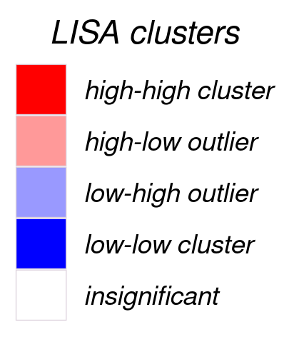
High-high and low-low clusters are areas with high or low value surrounded by areas with high or low value accordingly, indicating a statistically significant cluster of high or low values. High-low and low-high outliers are areas with high or low value surrounded by areas of low or high values accordingly, indicating statistically significant outliers.
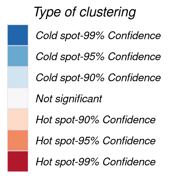
Getis-Ord Gi* (pronounced Gi-i-star) proposed by Getis and Ord in the mid 1990s is used to carry out hot spot analysis and identify tendency for negative and positive spatial clustering. Hot spots indicate significant clustering of high values while cold spots indicate significant clustering of low values. Areas in statistical significant hot spots have high values and are surrounded by other areas with high values.
Clustering is classified according to the following legend:
Kernel density computes the estimation of the intensity of a spatial phenomena in space. Computations were carried out on a spatial grid of 1000 x 1000 meters across the island, setting a distance threshold of 2500 meters inside of which another value can affect calculations and assuming an isotropic Gaussian kernel.
The above mentioned methods were studied more extensively by examining various settings of critical parameters and different types of visualizations.
Additionally for a more comprehensive study,not presented here, data from all three surveys 1572, 1832/33 and 1931 were spatially aggregated to the following regions as well as in those generated by spatial intersections of combinations of two sets from the following list:
- Administrative boundaries
- Bioclimatic regions
- Major Geographic regions
- Height zones
- Major drainage basins
- Geological formations
- Soil types according to the classification of the soil map of 1970